Devices in vipdopt
The Device class is how optical devices are represented in vipdopt. A Device object contains a 3D voxel-grid design region, with each voxel having its own refractive index, along with a number of helpful methods for interacting with the rest of the code library.
For later cells to work, please run the following block first.
[2]:
# imports
from pathlib import Path
import sys

import numpy as np
import matplotlib.pyplot as plt

np.set_printoptions(threshold=100)

# Get vipdopt directory path from Notebook
parent_dir = str(Path().resolve().parents[2])

# Add to sys.path
sys.path.insert(0, parent_dir)

# Imports from vipdopt
from vipdopt.optimization import Device, Sigmoid, Scale
from vipdopt.simulation import LumericalFDTD, LumericalSimulation, Source
from vipdopt.GDS import GDS
from vipdopt.STL import STL
Creating a Device
A Device requires a number of parameters to be created:
The size of the 3D-grid in voxels, given as a 3-tuple of integers
A Minimum and maximum permittivity
The coordinates of device in 3D space
This utilizes a
Coordinates, which is just a dictionary with ‘x’, ‘y’, and ‘z’
[4]:
device_size = (5, 5, 5) # use a 5x5x5 grid for the design region
permittivity_bounds = (0, 1)
# Center the device at the origin with a voxel size of 1
coords = {
'x': np.linspace(-2.5, 2.5, 5),
'y': np.linspace(-2.5, 2.5, 5),
'z': np.linspace(-2.5, 2.5, 5),
}
dev = Device(
device_size,
permittivity_bounds,
coords
)
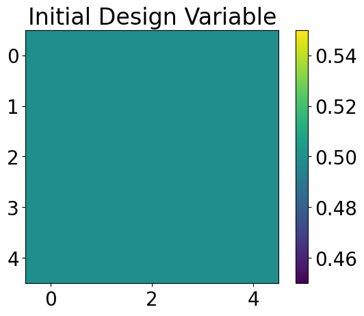
# By default the device will have density 0.5 everywhere
# Plot the design variable (the slice at z=0)
im = plt.imshow(dev.get_design_variable().real[..., 0])
plt.colorbar(im)
plt.title('Initial Design Variable')
[4]:
Text(0.5, 1.0, 'Initial Design Variable')
Optional Parameters
There are a number of optional parameters when creating a Device:
The name of the device (defaults to “device”)
A list of
FiltersInitialization parameters that are further described in the following section
Initialization Parameters
When creating a new device, there are a number of settings that can be tweaked to change the intital permittivity values it will be populated with
Initial Density
The initial density of the device is the parameter we are optimizing (frequently referred to as the “design variable”). It is then passed through Filters (possibly non-linearly) and then scaled to the permittivity contraints.
The init_density can be specified, or it defaults to 0.5. If randomize is False, the entire design varibale will be set uniformly to the initial density.
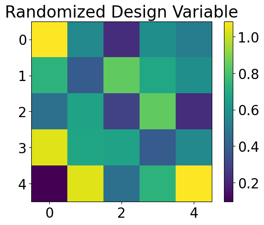
Randomization
If randomize is set to True, then the values will be drawn from a normal distribution centered at init_density, with scale 0.27.
A random seed can be specified by providing an integer. By default, the random seed is None which effectivley makes the seed random as well.
Symmetry
If symmetric is set to True the design variable will be symmetric over the line \(y=x\).
Miscellaneous Parameters
Additional paramerters can be passed into the Device using kwargs. These values won’t be used for any internal functionality in the Device but can be accessed as attributes if desired.
[3]:
# Make the device randomized and symmetric this time
dev = Device(
    device_size,
    permittivity_bounds,
    coords,
    randomize=True,
    symmetric=True
)

# Plot the design variable (the slice at z=0)
im = plt.imshow(dev.get_design_variable().real[..., 0])  # Plot first layer
plt.colorbar(im)
plt.title('Randomized Design Variable')
[3]:
Text(0.5, 1.0, 'Randomized Design Variable')
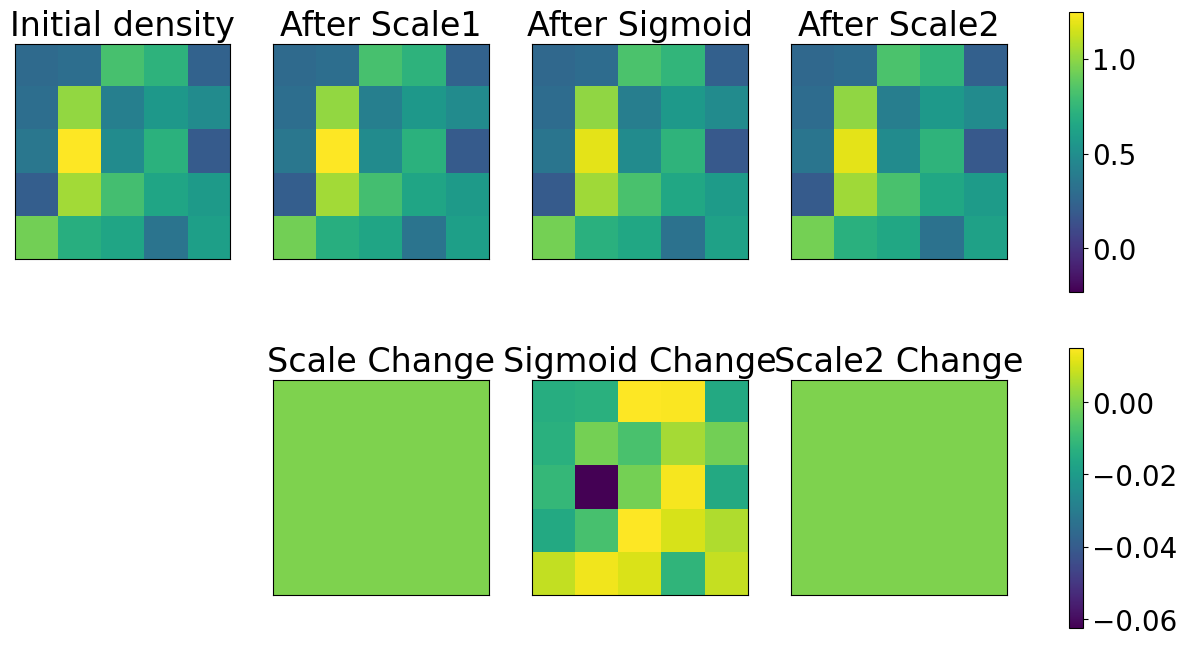
Filter
The Filter class is used to apply modifications to the design variable before converting to permittivity values. If you’re familiar with machine learning, Filters are analagous to activation functions.
A Filter is essentially three functions bundled together:
forward: passes an array through theFilter’s functionfabricate: similar toforwardbut binarizes array values for fabricationchain_rule: the gradient of theforwardfunction
There are two Filters included in vipdopt:
Sigmoidwhich applies a sigmoidal projection to push values to the 0/1 extremes.Scalewhich scales the input to a specified range
If a Device is created and there are no filters provided, or the last filter is not a Scale filter, a Scale filter will be appended to the end of the list with the permittivity constraints.
[4]:
sig_fil = Sigmoid(0.5, 1)
scale_fil = Scale((0, 1))

dev = Device(
    device_size,
    permittivity_bounds,
    coords,
    randomize=True,
    init_seed=5,
    filters=[scale_fil, sig_fil]
)
dev.update_density()

# Plot the initial density and after applying each filter
gridspec = {'width_ratios': [1, 1, 1, 1]}
fig, axes = plt.subplots(2, 4, sharey=True, figsize=(16, 8), gridspec_kw=gridspec)
fig.delaxes(axes[1, 0])

min_val = dev.w.min().real
max_val = dev.w.max().real
for i in range(4):
    im = axes[0, i].imshow(dev.w[..., 0, i].real, vmin=min_val, vmax=max_val)
    # axes[0, i].set_xlabel('x')
    # axes[0, i].set_aspect('equal')

axes[0, 0].set_title('Initial density')
# axes[0, 0].set_ylabel('y')
axes[0, 1].set_title('After Scale1')
axes[0, 2].set_title('After Sigmoid')
axes[0, 3].set_title('After Scale2')
fig.colorbar(im, ax=axes[0, :])

differences = np.diff(dev.w[..., 0, :]).real
for i in range(1, 4):
    im = axes[1, i].imshow(differences[..., i - 1], vmin=differences.min(), vmax=differences.max())
    # axes[0, i].set_xlabel('x')

# axes[1, 1].set_ylabel('y')

fig.colorbar(im, ax=axes[1, :])
axes[1, 1].set_title('Scale Change')
axes[1, 2].set_title('Sigmoid Change')
axes[1, 3].set_title('Scale2 Change')

for ax in axes.ravel():
    ax.set_xticks([])
    ax.set_yticks([])


# axs[0, 0].plot(dev.get_design_variable().real[..., 0])
# axs[0]
# plt.colorbar(im)
# plt.title('Randomized Design Variable')
Working with Simulations
Devices can be imported into LumericalSimulations. To do this, a LumericalSimulation must have an Import object to store the refractive index. Using Device.impurt_cur_index, the relevant values will be saved into the Import object until the simulation is loaded into Lumerical. For more details, see the notebook on simulations
The index may need to be reinterpolated to match the size of the voxel grid in Lumerical.
[5]:
# Set up simulation and get the Import object
sim = LumericalSimulation('simulation_example.json').with_enabled([Source('forward_src_x', 'gaussian')])
import_obj = sim.objects['design_import']

dev = Device(
    device_size,
    permittivity_bounds,
    coords,
    randomize=True,
    init_seed=0,
    filters=[Sigmoid(0.05, 0.5)],
)

# Store refractive index data in `import_obj`
_ = dev.import_cur_index(import_obj, reinterpolation_factor=1)

fdtd = LumericalFDTD()
fdtd.connect(hide=False)
fdtd.load_simulation(sim)  # This automatically imports the data stored in `import_obj`
C:\Users\tytym\Documents\Schmidt Academy\SonyBayerFilter\vipdopt\optimization\device.py:274: RuntimeWarning: invalid value encountered in sqrt
  return np.sqrt(np.real(permittivity))
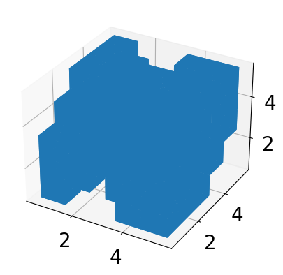
Exporting a Device
After an optimization, a finished Device can be exported to a .GDS or .STL file. The Device permittivity will also be binarized (all values will be converted to 0 or 1).
[18]:
dev = Device(
    device_size,
    permittivity_bounds,
    coords,
    randomize=True,
    init_seed=0,
    filters=[Sigmoid(0.05, 0.5)],
)

# ========= Export to STL ========
# STL Export requires density to be fully binarized
full_density = dev.binarize(dev.get_density())
stl_generator = STL(full_density)
stl_generator.generate_stl()
stl_generator.save_stl(dev.name + '.stl')
stl_generator.viz_stl()

# ======== Export to GDS =========

# GDS Export must be done in layers. We split the full design into individual
# layers, (not related to design layers). Express each layer as polygons in an
# STL Mesh object and write that layer into its own cell of the GDS file

layer_mesh_array = []
for z_layer in range(full_density.shape[2]):
    stl_generator = STL(full_density[..., z_layer][..., np.newaxis])
    stl_generator.generate_stl()
    layer_mesh_array.append(stl_generator.stl_mesh)

# Create a GDS object containing a Library with Cells corresponding to each 2D
# layer in the 3D device.
gds_generator = GDS.set_layers(
    full_density.shape[2],
    unit=1e-6
    * np.abs(dev.coords['x'][-1] - dev.coords['x'][0])
    / dev.size[0],
)
gds_generator.assemble_device(layer_mesh_array, listed=False)
gds_generator.export_device('.', filetype='gds')